Pytorch实现GCN(基于Message Passing消息传递机制实现)

2023-02-28

self data gcn

文章目录前言一、导入相关库二、加载Cora数据集三、定义GCN网络3.1定义GCN层3.1.1消息传递阶段（message）3.1.2消息聚合阶段（aggregate）3.1.3节点更新阶段（update）3.1.4定义传播过程（propagate）3.1.5定义GCNConv层3.2定义GCN网络

文章目录

前言
一、导入相关库
二、加载Cora数据集
三、定义GCN网络
- 3.1 定义GCN层
- - 3.1.1 消息传递阶段（message）
  - 3.1.2 消息聚合阶段（aggregate）
  - 3.1.3 节点更新阶段（update）
  - 3.1.4 定义传播过程（propagate）
  - 3.1.5 定义GCNConv层
- 3.2 定义GCN网络
四、定义模型
五、模型训练
六、模型验证
七、结果
完整代码

前言

大家好，我是阿光。

本专栏整理了《图神经网络代码实战》，内包含了不同图神经网络的相关代码实现（PyG以及自实现），理论与实践相结合，如GCN、GAT、GraphSAGE等经典图网络，每一个代码实例都附带有完整的代码。

正在更新中~ ✨

🚨 我的项目环境：

平台：Windows10
语言环境：python3.7
编译器：PyCharm
PyTorch版本：1.11.0
PyG版本：2.1.0

💥 项目专栏：【图神经网络代码实战目录】

本文我们将使用PyTorch来简易实现一个GCN（图卷积网络），不使用PyG库，让新手可以理解如何PyTorch来搭建一个简易的图网络实例demo。

一、导入相关库

本项目是采用自己实现的GCN，使用的是 图神经网络生成节点表征的范式–消息传递（Message Passing）范式，它将卷积算子推广到了不规则数据领域，实现了图与神经网络的连接，消息传递范式由于简单、强大的特性，现已被人们广泛地使用。

import numpy as np
import torch
import torch.nn as nn
import torch.nn.functional as F
import torch_geometric.nn as pyg_nn
from torch_geometric.nn import MessagePassing
from torch_scatter import scatter
from torch_geometric.utils import add_self_loops, degree
from scipy.sparse import coo_matrix
from torch_geometric.datasets import Planetoid
1
2
3
4
5
6
7
8
9
10

二、加载Cora数据集

本文使用的数据集是比较经典的Cora数据集，它是一个根据科学论文之间相互引用关系而构建的Graph数据集合，论文分为7类，共2708篇。

Genetic_Algorithms
Neural_Networks
Probabilistic_Methods
Reinforcement_Learning
Rule_Learning
Theory

这个数据集是一个用于图节点分类的任务，数据集中只有一张图，这张图中含有2708个节点，10556条边，每个节点的特征维度为1433。

# 1.加载Cora数据集
dataset = Planetoid(root='./data/Cora', name='Cora')
1
2

三、定义GCN网络

3.1 定义GCN层

这里我们就不重点介绍GCN网络了，相信大家能够掌握基本原理，本文我们使用的是PyTorch定义网络层。

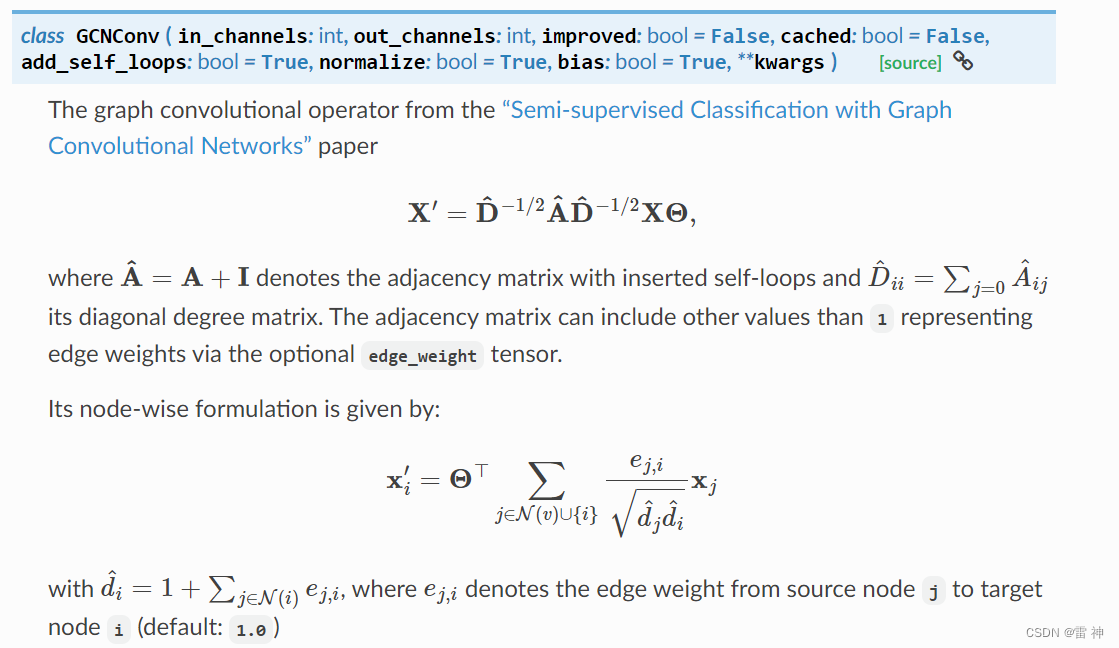
对于GCNConv的常用参数：

in_channels：每个样本的输入维度，就是每个节点的特征维度
out_channels：经过 GCNConv 后映射成的新的维度，就是经过 GCNConv 后每个节点的维度长度
add_self_loops：为图添加自环，是否考虑自身节点的信息
bias：训练一个偏置b

我们在实现时也是考虑这几个常见参数

对于GCN的传播公式为：
$H'=\hat D^{-1/2} \hat A \hat D^{-1/2}HW$

上式子中的 $D$ 代表图的度矩阵， $A$ 代表邻接矩阵，如果考虑自身特征，则 $\hat A=A+I$ ， $H$ 代表每个层的输入特征，也就是每个节点的特征矩阵，如果是第一层，则 $H_0=X$ ，对于 $W$ 代表每个 GCNConv 层的可学习参数。

对于消息传递图神经网络可以描述为：
$x_i^{k}=\gamma^{k}(x_i^{k-1},□_{j\in N(i)},\phi^{k}(x_i^{k-1},x_j^{k-1},e_{j,i}))$

关于消息传递具体的介绍，可以百度了解，本文注重实战部分，所以理论就不再赘述，对于本项目搭建的是GCN网络，下文基于消息传递机制来实现GCN。

3.1.1 消息传递阶段（message）

对于消息传递阶段就是对所有的节点特征进行映射，也就是对应上式的 $\phi$ 函数，在GCN中我们需要对所有的节点进行新的维度映射，然后再使用度矩阵将其归一化。

def message(self, x, edge_index):
# 1.对所有节点进行新的空间映射
x = self.linear(x) # [num_nodes, feature_size]

# 2.添加偏置
if self.bias != None:
    x += self.bias.flatten()

# 3.返回source、target信息，对应边的起点和终点
row, col = edge_index # [E]

# 4.获得度矩阵
deg = degree(col, x.shape[0], x.dtype) # [num_nodes]

# 5.度矩阵归一化
deg_inv_sqrt = deg.pow(-0.5) # [num_nodes]

# 6.计算sqrt(deg(i)) * sqrt(deg(j))
norm = deg_inv_sqrt[row] * deg_inv_sqrt[col] # [num_edges]

# 7.返回所有边的映射
x_j = x[row] # [E, feature_size]

# 8.计算归一化后的节点特征
x_j = norm.view(-1, 1) * x_j # [E, feature_size]

return x_j
1
2
3
4
5
6
7
8
9
10
11
12
13
14
15
16
17
18
19
20
21
22
23
24
25
26
27

3.1.2 消息聚合阶段（aggregate）

对于消息聚合阶段的输入参数就是消息传递的输出，在这个阶段我们会将目标节点的邻居特征进行聚合操作，在GCN中，消息聚合采用的方式是求和 sum，简单实现我们使用的是 PyG 工具类中提供的 scatter() 函数。

def aggregate(self, x_j, edge_index):
# 1.返回source、target信息，对应边的起点和终点
row, col = edge_index # [E]

# 2.聚合邻居特征
aggr_out = scatter(x_j, col, dim=0, reduce='sum') # [num_nodes, feature_size]

return aggr_out
1
2
3
4
5
6
7
8

3.1.3 节点更新阶段（update）

正常来讲，节点更新阶段是将目标节点的特征信息与上一阶段聚合后的邻居特征进行进一步的处理来作为目标节点的特征。

但是GCN网络中没有这个阶段，所以直接将输入返回即可

def update(self, aggr_out):
# 对于GCN没有这个阶段，所以直接返回
return aggr_out
1
2
3

3.1.4 定义传播过程（propagate）

定义好三个函数，我们需要在forward中进行调用，但是我们的类已经继承了 MessagePassing 这个基类，这个类中已经实现好了 propagate() 函数，这个函数会依次顺序调用 message() 、aggregate() 、update() 这三个函数，所以我们可以直接在forward中调用父类的 propagate() 函数即可。

def forward(self, x, edge_index):
# 2.添加自环信息，考虑自身信息
if self.add_self_loops:
    edge_index, _ = add_self_loops(edge_index, num_nodes=x.shape[0]) # [2, E]

return self.propagate(edge_index, x=x)
1
2
3
4
5
6

如果不继承 MessagePassing 这个基类，可以自己实现一个方法来依次调用我们定义好的传递函数，代码如下：

def propagate(self, x, edge_index):
x_j = self.message(x, edge_index)
aggr_out = self.aggregate(x_j, edge_index)
output = self.update(aggr_out, edge_index)

return output
1
2
3
4
5
6

这种实现方法实现相对MessagePassing实现好的相对简略，但是保留了基本逻辑

3.1.5 定义GCNConv层

定义GCNConv层的代码如下：

# 2.定义GCNConv层
class GCNConv(MessagePassing):
    def __init__(self, in_channels, out_channels, add_self_loops=True, bias=True):
        super(GCNConv, self).__init__()
        self.add_self_loops = add_self_loops
        self.edge_index = None
        self.linear = pyg_nn.dense.linear.Linear(in_channels, out_channels, weight_initializer='glorot')
        
        
        if bias:
            self.bias = nn.Parameter(torch.Tensor(out_channels, 1))
            self.bias = pyg_nn.inits.glorot(self.bias)
        else:
            self.register_parameter('bias', None)
    
    # 1.消息传递
    def message(self, x, edge_index):
        # 1.对所有节点进行新的空间映射
        x = self.linear(x) # [num_nodes, feature_size]
        
        # 2.添加偏置
        if self.bias != None:
            x += self.bias.flatten()
        
        # 3.返回source、target信息，对应边的起点和终点
        row, col = edge_index # [E]
        
        # 4.获得度矩阵
        deg = degree(col, x.shape[0], x.dtype) # [num_nodes]
        
        # 5.度矩阵归一化
        deg_inv_sqrt = deg.pow(-0.5) # [num_nodes]
        
        # 6.计算sqrt(deg(i)) * sqrt(deg(j))
        norm = deg_inv_sqrt[row] * deg_inv_sqrt[col] # [num_nodes]
        
        # 7.返回所有边的映射
        x_j = x[row] # [E, feature_size]
        
        # 8.计算归一化后的节点特征
        x_j = norm.view(-1, 1) * x_j # [E, feature_size]
        
        return x_j
    
    # 2.消息聚合
    def aggregate(self, x_j, edge_index):
        # 1.返回source、target信息，对应边的起点和终点
        row, col = edge_index # [E]
        
        # 2.聚合邻居特征
        aggr_out = scatter(x_j, row, dim=0, reduce='sum') # [num_nodes, feature_size]
        
        return aggr_out
    
    # 3.节点更新
    def update(self, aggr_out):
        # 对于GCN没有这个阶段，所以直接返回
        return aggr_out
    
    def forward(self, x, edge_index):
        # 2.添加自环信息，考虑自身信息
        if self.add_self_loops:
            edge_index, _ = add_self_loops(edge_index, num_nodes=x.shape[0]) # [2, E]
        
        return self.propagate(edge_index, x=x)
1
2
3
4
5
6
7
8
9
10
11
12
13
14
15
16
17
18
19
20
21
22
23
24
25
26
27
28
29
30
31
32
33
34
35
36
37
38
39
40
41
42
43
44
45
46
47
48
49
50
51
52
53
54
55
56
57
58
59
60
61
62
63
64
65

3.2 定义GCN网络

上面我们已经实现好了 GCNConv 的网络层，之后就可以调用这个层来搭建 GCN 网络。

# 定义GCN网络
class GCN(nn.Module):
    def __init__(self, num_node_features, num_classes):
        super(GCN, self).__init__()
        self.conv1 = GCNConv(num_node_features, 16)
        self.conv2 = GCNConv(16, num_classes)
        
    def forward(self, data):
        x, edge_index = data.x, data.edge_index
        
        x = self.conv1(x, edge_index)
        x = F.relu(x)
        x = F.dropout(x, training=self.training)
        x = self.conv2(x, edge_index)
        
        return F.log_softmax(x, dim=1)
1
2
3
4
5
6
7
8
9
10
11
12
13
14
15
16

上面网络我们定义了两个GCNConv层，第一层的参数的输入维度就是初始每个节点的特征维度，输出维度是16。

第二个层的输入维度为16，输出维度为分类个数，因为我们需要对每个节点进行分类，最终加上softmax操作。

四、定义模型

下面就是定义了一些模型需要的参数，像学习率、迭代次数这些超参数，然后是模型的定义以及优化器及损失函数的定义，和pytorch定义网络是一样的。

device = torch.device('cuda' if torch.cuda.is_available() else 'cpu') # 设备
epochs = 10 # 学习轮数
lr = 0.003 # 学习率
num_node_features = dataset.num_node_features # 每个节点的特征数
num_classes = dataset.num_classes # 每个节点的类别数
data = dataset[0].to(device) # Cora的一张图

# 3.定义模型
model = GCN(num_node_features, num_classes).to(device)
optimizer = torch.optim.Adam(model.parameters(), lr=lr) # 优化器
loss_function = nn.NLLLoss() # 损失函数
1
2
3
4
5
6
7
8
9
10
11

五、模型训练

模型训练部分也是和pytorch定义网络一样，因为都是需要经过前向传播、反向传播这些过程，对于损失、精度这些指标可以自己添加。

# 训练模式
model.train()

for epoch in range(epochs):
    optimizer.zero_grad()
    pred = model(data)
    
    loss = loss_function(pred[data.train_mask], data.y[data.train_mask]) # 损失
    correct_count_train = pred.argmax(axis=1)[data.train_mask].eq(data.y[data.train_mask]).sum().item() # epoch正确分类数目
    acc_train = correct_count_train / data.train_mask.sum().item() # epoch训练精度
    
    loss.backward()
    optimizer.step()
    
    if epoch % 20 == 0:
        print("【EPOCH: 】%s" % str(epoch + 1))
        print('训练损失为：{:.4f}'.format(loss.item()), '训练精度为：{:.4f}'.format(acc_train))

print('【Finished Training！】')
1
2
3
4
5
6
7
8
9
10
11
12
13
14
15
16
17
18
19

六、模型验证

下面就是模型验证阶段，在训练时我们是只使用了训练集，测试的时候我们使用的是测试集，注意这和传统网络测试不太一样，在图像分类一些经典任务中，我们是把数据集分成了两份，分别是训练集、测试集，但是在Cora这个数据集中并没有这样，它区分训练集还是测试集使用的是掩码机制，就是定义了一个和节点长度相同纬度的数组，该数组的每个位置为True或者False，标记着是否使用该节点的数据进行训练。

# 模型验证
model.eval()
pred = model(data)

# 训练集（使用了掩码）
correct_count_train = pred.argmax(axis=1)[data.train_mask].eq(data.y[data.train_mask]).sum().item()
acc_train = correct_count_train / data.train_mask.sum().item()
loss_train = loss_function(pred[data.train_mask], data.y[data.train_mask]).item()

# 测试集
correct_count_test = pred.argmax(axis=1)[data.test_mask].eq(data.y[data.test_mask]).sum().item()
acc_test = correct_count_test / data.test_mask.sum().item()
loss_test = loss_function(pred[data.test_mask], data.y[data.test_mask]).item()

print('Train Accuracy: {:.4f}'.format(acc_train), 'Train Loss: {:.4f}'.format(loss_train))
print('Test  Accuracy: {:.4f}'.format(acc_test), 'Test  Loss: {:.4f}'.format(loss_test))
1
2
3
4
5
6
7
8
9
10
11
12
13
14
15
16

七、结果

【EPOCH: 】1
训练损失为：1.9976 训练精度为：0.1786
【EPOCH: 】21
训练损失为：1.9102 训练精度为：0.2571
【EPOCH: 】41
训练损失为：1.8227 训练精度为：0.3286
【EPOCH: 】61
训练损失为：1.7244 训练精度为：0.3643
【EPOCH: 】81
训练损失为：1.6550 训练精度为：0.4929
【EPOCH: 】101
训练损失为：1.5842 训练精度为：0.5143
【EPOCH: 】121
训练损失为：1.4947 训练精度为：0.6143
【EPOCH: 】141
训练损失为：1.4328 训练精度为：0.6571
【EPOCH: 】161
训练损失为：1.3157 训练精度为：0.7857
【EPOCH: 】181
训练损失为：1.2323 训练精度为：0.7286
【Finished Training！】

>>>Train Accuracy: 0.9857 Train Loss: 1.0022
>>>Test  Accuracy: 0.4580 Test  Loss: 1.6971
1
2
3
4
5
6
7
8
9
10
11
12
13
14
15
16
17
18
19
20
21
22
23
24

	训练集	测试集
Accuracy	0.9857	0.4580
Loss	1.0022	1.6971

完整代码

import numpy as np
import torch
import torch.nn as nn
import torch.nn.functional as F
import torch_geometric.nn as pyg_nn
from torch_geometric.nn import MessagePassing
from torch_scatter import scatter
from torch_geometric.utils import add_self_loops, degree
from scipy.sparse import coo_matrix
from torch_geometric.datasets import Planetoid

# 1.加载Cora数据集
dataset = Planetoid(root='./data/Cora', name='Cora')

# 2.定义GCNConv层
class GCNConv(MessagePassing):
    def __init__(self, in_channels, out_channels, add_self_loops=True, bias=True):
        super(GCNConv, self).__init__()
        self.add_self_loops = add_self_loops
        self.edge_index = None
        self.linear = pyg_nn.dense.linear.Linear(in_channels, out_channels, weight_initializer='glorot')
        
        
        if bias:
            self.bias = nn.Parameter(torch.Tensor(out_channels, 1))
            self.bias = pyg_nn.inits.glorot(self.bias)
        else:
            self.register_parameter('bias', None)
    
    # 1.消息传递
    def message(self, x, edge_index):
        # 1.对所有节点进行新的空间映射
        x = self.linear(x) # [num_nodes, feature_size]
        
        # 2.添加偏置
        if self.bias != None:
            x += self.bias.flatten()
        
        # 3.返回source、target信息，对应边的起点和终点
        row, col = edge_index # [E]
        
        # 4.获得度矩阵
        deg = degree(col, x.shape[0], x.dtype) # [num_nodes]
        
        # 5.度矩阵归一化
        deg_inv_sqrt = deg.pow(-0.5) # [num_nodes]
        
        # 6.计算sqrt(deg(i)) * sqrt(deg(j))
        norm = deg_inv_sqrt[row] * deg_inv_sqrt[col] # [num_nodes]
        
        # 7.返回所有边的映射
        x_j = x[row] # [E, feature_size]
        
        # 8.计算归一化后的节点特征
        x_j = norm.view(-1, 1) * x_j # [E, feature_size]
        
        return x_j
    
    # 2.消息聚合
    def aggregate(self, x_j, edge_index):
        # 1.返回source、target信息，对应边的起点和终点
        row, col = edge_index # [E]
        
        # 2.聚合邻居特征
        aggr_out = scatter(x_j, row, dim=0, reduce='sum') # [num_nodes, feature_size]
        
        return aggr_out
    
    # 3.节点更新
    def update(self, aggr_out):
        # 对于GCN没有这个阶段，所以直接返回
        return aggr_out
    
    def forward(self, x, edge_index):
        # 2.添加自环信息，考虑自身信息
        if self.add_self_loops:
            edge_index, _ = add_self_loops(edge_index, num_nodes=x.shape[0]) # [2, E]
        
        return self.propagate(edge_index, x=x)

# 3.定义GCNConv网络
class GCN(nn.Module):
    def __init__(self, num_node_features, num_classes):
        super(GCN, self).__init__()
        self.conv1 = GCNConv(num_node_features, 16)
        self.conv2 = GCNConv(16, num_classes)
        
    def forward(self, data):
        x, edge_index = data.x, data.edge_index
        
        x = self.conv1(x, edge_index)
        x = F.relu(x)
        x = F.dropout(x, training=self.training)
        x = self.conv2(x, edge_index)
        
        return F.log_softmax(x, dim=1)

device = torch.device('cuda' if torch.cuda.is_available() else 'cpu') # 设备
epochs = 200 # 学习轮数
lr = 0.0003 # 学习率
num_node_features = dataset.num_node_features # 每个节点的特征数
num_classes = dataset.num_classes # 每个节点的类别数
data = dataset[0].to(device) # Cora的一张图

# 4.定义模型
model = GCN(num_node_features, num_classes).to(device)
optimizer = torch.optim.Adam(model.parameters(), lr=lr) # 优化器
loss_function = nn.NLLLoss() # 损失函数

# 训练模式
model.train()

for epoch in range(epochs):
    optimizer.zero_grad()
    pred = model(data)
    
    loss = loss_function(pred[data.train_mask], data.y[data.train_mask]) # 损失
    correct_count_train = pred.argmax(axis=1)[data.train_mask].eq(data.y[data.train_mask]).sum().item() # epoch正确分类数目
    acc_train = correct_count_train / data.train_mask.sum().item() # epoch训练精度
    
    loss.backward()
    optimizer.step()
    
    if epoch % 20 == 0:
        print("【EPOCH: 】%s" % str(epoch + 1))
        print('训练损失为：{:.4f}'.format(loss.item()), '训练精度为：{:.4f}'.format(acc_train))

print('【Finished Training！】')

# 模型验证
model.eval()
pred = model(data)

# 训练集（使用了掩码）
correct_count_train = pred.argmax(axis=1)[data.train_mask].eq(data.y[data.train_mask]).sum().item()
acc_train = correct_count_train / data.train_mask.sum().item()
loss_train = loss_function(pred[data.train_mask], data.y[data.train_mask]).item()

# 测试集
correct_count_test = pred.argmax(axis=1)[data.test_mask].eq(data.y[data.test_mask]).sum().item()
acc_test = correct_count_test / data.test_mask.sum().item()
loss_test = loss_function(pred[data.test_mask], data.y[data.test_mask]).item()

print('Train Accuracy: {:.4f}'.format(acc_train), 'Train Loss: {:.4f}'.format(loss_train))
print('Test  Accuracy: {:.4f}'.format(acc_test), 'Test  Loss: {:.4f}'.format(loss_test))
1
2
3
4
5
6
7
8
9
10
11
12
13
14
15
16
17
18
19
20
21
22
23
24
25
26
27
28
29
30
31
32
33
34
35
36
37
38
39
40
41
42
43
44
45
46
47
48
49
50
51
52
53
54
55
56
57
58
59
60
61
62
63
64
65
66
67
68
69
70
71
72
73
74
75
76
77
78
79
80
81
82
83
84
85
86
87
88
89
90
91
92
93
94
95
96
97
98
99
100
101
102
103
104
105
106
107
108
109
110
111
112
113
114
115
116
117
118
119
120
121
122
123
124
125
126
127
128
129
130
131
132
133
134
135
136
137
138
139
140
141
142
143
144
145

文章知识点与官方知识档案匹配，可进一步学习相关知识

Python入门技能树人工智能深度学习237982 人正在系统学习中

AI人工智能研习社

微信公众号

主要分享前沿的论文动态

深圳幻海软件技术有限公司

Pytorch实现GCN(基于Message Passing消息传递机制实现)

文章目录

前言

一、导入相关库

二、加载Cora数据集

三、定义GCN网络

3.1 定义GCN层

3.1.1 消息传递阶段（message）

3.1.2 消息聚合阶段（aggregate）

3.1.3 节点更新阶段（update）

3.1.4 定义传播过程（propagate）

3.1.5 定义GCNConv层

3.2 定义GCN网络

四、定义模型

五、模型训练

六、模型验证

七、结果

完整代码

程序狗必备：5个功能丰富的交互式Javascript库

终于明白为什么要加 final 关键字了！

Battle！用JavaScript发出HTTP请求的不同方法

IOC-Golang 的 AOP 原理与应用

健康的Ceph 集群需要避免的16种操作

微信iOS推送8.0.15版更新：后台频繁读取相册功能已停用

明修"栈"道——越过Android启动栈陷阱

linux命令行之c文件从制作到执行

深圳幻海软件技术有限公司

Pytorch实现GCN(基于Message Passing消息传递机制实现)

文章目录

前言

一、导入相关库

二、加载Cora数据集

三、定义GCN网络

3.1 定义GCN层

3.1.1 消息传递阶段（message）

3.1.2 消息聚合阶段（aggregate）

3.1.3 节点更新阶段（update）

3.1.4 定义传播过程（propagate）

3.1.5 定义GCNConv层

3.2 定义GCN网络

四、定义模型

五、模型训练

六、模型验证

七、结果

完整代码

ACM基础(一)

国产数据库，又有好消息！